


In a previous blogpost [see “How many devs fit on a GPU?”], we studied how many developers can use a common LLM inference engine effectively without slowing down the GPU system to a crawl… and of course, the answer is “it depends”. The basic mechanics at play are worth an article on their own. In this article, our goal is to give you a back-of-the-napkin understanding of why a single-user chat session is barely noticed by your GPU, but a few long-context agentic coding sessions can make it break a sweat.
Tokens, caches, batches
and all that
A language model does one thing — predict the next token — then feeds each new word back in and does it again. Everything about fitting one on a GPU comes down to serving that sequential loop: what it recomputes, what it caches, and how much it has to move each step.
Autoregressive Large Language Models (LLMs) do exactly one thing: generating text. An LLM does this probabilistically, and exactly one word at a time: given the preceding sequence of words, the context, it produces a probability distribution over what it believes the next word should be. Feed it “Once upon a midnight” as context and it will — remembering Poe [1] — output a distribution with a high probability for “dreary”. Sample a word from that distribution (big chance it will be “dreary”), append it to the context, and run everything again to generate the word after “dreary”. Repeat until done.
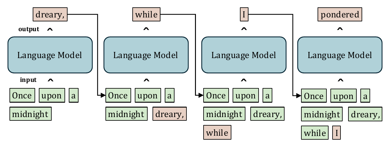
Autoregressive generation: one token at a time
To be precise, LLMs don’t operate on words, but on tokens. Tokens are chunks that may be any combination of (sub)-words, spaces, punctuation, symbols, etc. Sequences of these tokens can represent text from many natural and programming languages using a single unified vocabulary. Everything we provide as context is first converted into tokens, everything the LLM generates needs to be converted back into text before we read it. This is why many of the metrics we use (e.g. tokens per second) measure tokens instead of words.
As explained, longer texts are generated by repeatedly invoking the model, one token at a time. Naively, every generation step would process the entire (growing) context again from scratch. Nobody does that, because it would saturate your GPUs just to keep repeating the same computations on the same input. For this reason, intermediate results for processed tokens in the context are stored for reuse in the KV cache. Each generation step simply reads from that KV cache instead of churning through the same context repeatedly.
Initially, there is no KV cache yet to read from. The model has to process the whole input prompt at once to build up the KV cache and generate a single output token. This is called prefill. From there on, every subsequent step, called decode, just feeds the newest token as input to the model. Only this input token is processed, while the information associated with previous tokens is read from the KV cache. As in prefill, every decode step produces a single output token. Additionally, the KV cache is updated with the intermediate results of every added token.
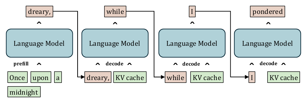
Prefill builds the cache, decode reads it
In short. Prefill: process the whole prompt once, build the KV cache, and produce a single output token. Decode: process one token, read KV cache, append token to the KV cache, and produce a single output token. Rinse and repeat.
LLMs often receive multiple requests at once, each with its own context. The number of such concurrent sequences is the batch size. In each decode step the model then generates one new token per sequence. Each sequence still drags along its own KV cache — an important detail for later.
Introducing the
Roofline model
Every operation runs into one of two ceilings — how fast the hardware can move data, or how fast it can compute. Which one you hit sets your speed, and for generating tokens it’s almost always memory bandwidth, not raw FLOPs.
When you send a request to Claude, where does the processing time go while you sip from a freshly brewed coffee? AI is mostly just linear algebra so most of the time goes into matrix multiplications. To reason about them, we use a well established tool: the roofline model. It tells us that the runtime of any operation is limited by one of two ceilings: how fast you can move data around (memory bandwidth) and how fast you can crunch it (peak FLOPs/s).
Take a simple vector-addition as an example. Let’s say both vectors are \(10^{9}\) elements long, with each element taking up 2 bytes. We would need to — at least — read both vectors (\(2\times10^{9}\) bytes), do the additions (= \(10^{9}\) FLOPs) and write back the result (another \(2\times10^{9}\) bytes), so \(6\times10^{9}\) bytes in total. On an NVIDIA B200, with a peak computation speed of \(C_{peak}\approx2.25\times10^{15}\) FLOPs/s, the compute would take at minimum \(T_{comp}=10^{9}/C_{peak}\approx0.44\,\text{ms}\). With its HBM4 bandwidth of \(B_{mem}\approx8\times10^{12}\) bytes/s, moving the data would take \(T_{mem}=6\times10^{9}/B_{mem}\approx75\,\text{ms}\).
Just take a moment here to appreciate the marvel of engineering: with this \(B_{mem}\), we can read the equivalent of about 11000 CD-ROMs every second. Those would stack 13 meters high!
You may think those act serially, data is moved, processed and moved again. But modern hardware is optimized to overlap data transfers and compute. A better — although still idealized — estimate of the total run time is to model it as whichever of the two takes the longest: \(T_{total}=\max(T_{mem},T_{comp})\). In this example, \(T_{mem}\gg T_{comp}\), i.e. we are memory-bandwidth-bound. Being memory-bandwidth-bound is usually bad news. It means your expensive accelerator’s compute units are idling, waiting for data to arrive. We’d rather be compute-bound instead; this is when \(T_{comp}\) dominates. Only then are we getting out of the hardware what we paid for.
To make this happen, we need our operations to perform a lot of FLOPs for every byte of data transferred: \(C_{peak}/B_{mem}\) FLOPs per byte to be specific. This is approximately 280 FLOPs per byte on a B200. In other words, run time is bottlenecked by memory bandwidth unless we use operations which can heavily reuse each byte they load into memory.
The table below compiles the FLOPs per byte for some example operations (at 2 bytes per element). The takeaway here is that big matrix-matrix multiplies give you lots of computational bang for your memory bandwidth buck — operations on vectors don’t. The former are compute-bound, working with the latter will be bottlenecked on memory bandwidth.
| Operation | Operand sizes | FLOPs | Bytes | FLOPs per byte | Regime |
|---|---|---|---|---|---|
| vector-addition | \([4096]+[4096]\) | \(4.1\times10^{3}\) | 24 KB | 0.17 | memory-bandwidth-bound |
| dot product | \([4096]\cdot[4096]\) | \(8.2\times10^{3}\) | 16 KB | 0.5 | memory-bandwidth-bound |
| outer product | \([4096]\otimes[4096]\) | \(1.7\times10^{7}\) | 32 MB | 0.5 | memory-bandwidth-bound |
| matrix-vector multiplication | \([4096,4096]\cdot[4096]\) | \(3.4\times10^{7}\) | 32 MB | 1 | memory-bandwidth-bound |
| matrix-matrix multiplication | \([4096,4096]\cdot[4096,4096]\) | \(1.4\times10^{11}\) | 96 MB | 1365 | compute-bound |
Inside the
Transformer
A Transformer is a stack of two repeating parts: attention, which lets each token look back at the ones before it, and a feed-forward network, which holds most of the model’s knowledge. Their very different compute and memory demands are what the whole performance picture is built on.
The roofline model allows us to estimate the runtime of matrix-matrix and matrix-vector multiplications. To a large extent, LLM inference can be decomposed into a sequence of such operations. Their matrix shapes depend on whether the model is performing prefill or decode, on the number of concurrent users (batch size), and on the context length. These shapes, in turn, determine whether each operation is limited by memory bandwidth or compute performance. To estimate the total runtime of LLM inference, we must therefore identify the relevant operations and their dimensions.
Most modern LLM models are Transformers: a stack of identical layers, each doing two different things. An Attention Mechanism lets every token pull in information from the tokens before it. This helps with grammar, long-range reference and context in general. A Feed-Forward Network (FFN) then processes each token independently and contributes much of the model’s linguistic and factual knowledge. Every token travels through the stack as a vector of numbers up until the last layer. There, the final token’s vector becomes a probability distribution over the token vocabulary. From this distribution, the next token is sampled.

We now discuss both the Feed Forward Network and the Attention Mechanism in more detail. We focus solely on whether the computations involved are memory-bandwidth-bound or compute-bound. For more details on the inner workings of the FFN and Attention Mechanism, we refer to [INSERT EXCELLENT REFERENCE — e.g. “How to build an LLM from scratch” by Sebastian Raschka].
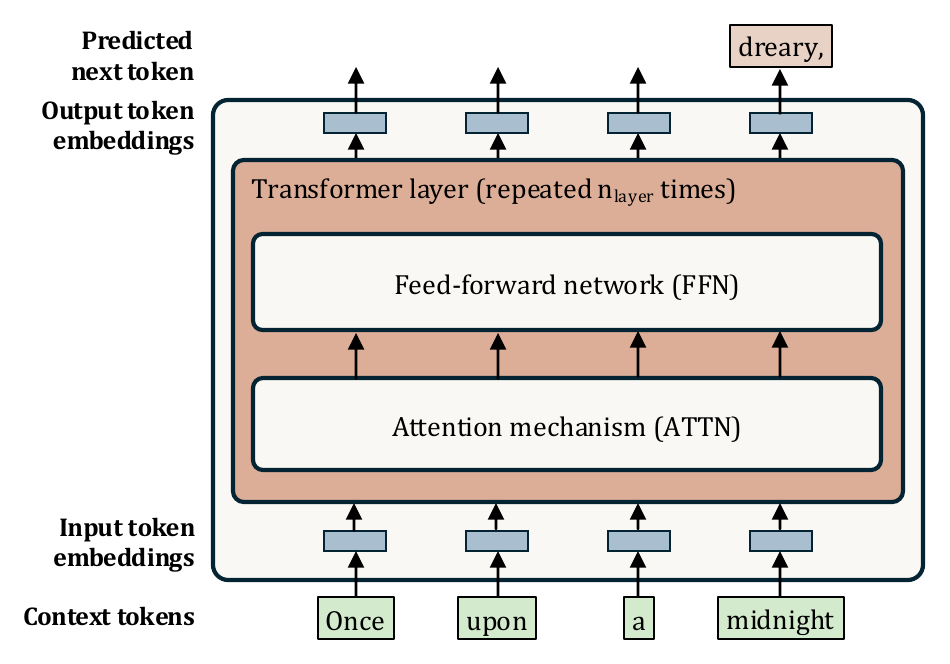
Inside the Transformer: a stack of identical layers
The Feed Forward Network
There exist many different FFN architectures, nowadays a popular option is the SwiGLU-FFN (Swish-Gated Linear Unit). As you can see from the diagram, it looks quite complex.
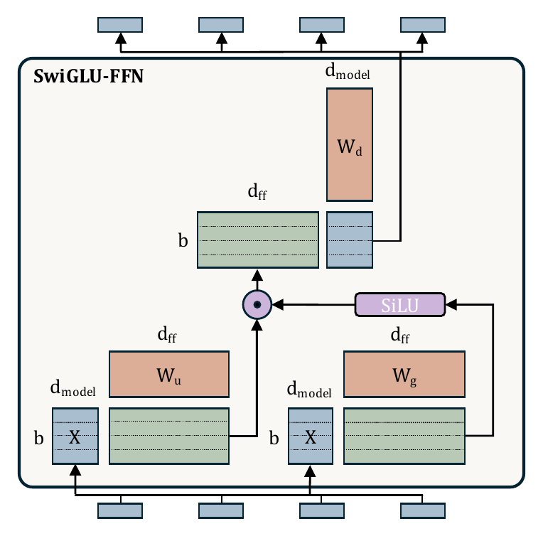
The SwiGLU feed-forward network
From a roofline perspective, all that matters are the three matrix-matrix multiplications, indicated by \(\ast\) in the formula. The element-wise operations (\(\text{SiLU}, \odot\)) are cheap in comparison and can be ignored. To estimate the runtime of the FFN using the roofline model, we just need to understand the dimensions of the matrices involved.
The dimensions of the weight matrices \(W\) are dictated by the model architecture and thus fixed. They are relatively large: for the Llama3-8B model, the dimensions are 4096 by 14336 for \(W_{gate}\) and \(W_{up}\) and 14336 by 4096 for \(W_{down}\). The \(X\) matrix is obtained by stacking the \(b\) input tokens. We can do this because the FFN is applied to each input token independently, without interaction between tokens. In the context of the FFN, it therefore does not matter whether these \(b\) tokens belong to the same sequence, or to different users. For Llama3-8B, the \(X\) matrix has dimensions \(b\) by 4096.
Therefore, the FFN’s fate is solely determined by \(b\): in case of a single-user decode scenario \((b=1)\), \(X\) is a vector. All operations are then memory-bandwidth-bound matrix-vector multiplications. In contrast, if \(b\) is large enough (prefill or batched decode), the FFN’s main computations are matrix-matrix multiplications, which run at near-peak compute performance.
| Situation | Value of \(b\) | Typical FFN regime |
|---|---|---|
| Single-user decode | \(b=1\) | memory-bandwidth-bound |
| Batched decoding, many users | \(b\gg1\) | compute-bound |
| Prefill for long prompt(s) | \(b\gg1\) | compute-bound |
Great! The FFN is almost always using our shiny, expensive GPUs effectively! But now let’s turn our attention to the other child, the attention mechanism.
The Attention Mechanism
This is the place in the transformer where tokens within the same sequence talk to each other. As our working example, we’ll examine a vanilla multi-head attention. The architecture is unquestionably even more complex than that of the FFN. But again, looking through the lens of the roofline model, we can abstract much of it. It is also where prefill and decode part ways and we therefore discuss them separately.
The Attention Mechanism: Prefill
In the case of prefill, the input consists of \(b\) prompt tokens that belong to the same sequence. As for the FFN, their vector representations are stacked to form input matrix \(X\).
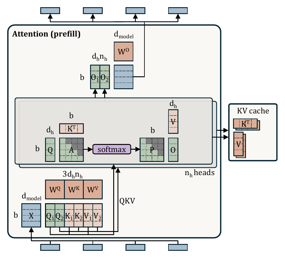
Attention during prefill
Again, we spend a considerable part of our compute on multiplying our input matrix \(X\) with weight matrices \(W^{Q}\), \(W^{K}\), and \(W^{V}\) for the input projections. Unless the prompt length is very short, those operations are easily compute-bound. Using a similar reasoning, the output projection with weight matrix \(W^{O}\) is compute-bound.
Apart from those projections, we also have multiple attention heads, each computing an attention operation \(O = \text{softmax}(Q \ast K^{T}) \ast V\). Unlike the projections, in which we multiplied activations with model weights, we are now multiplying activations with each other. This is where tokens exchange information with each other. But those are still genuine matrix-matrix multiplications with great FLOPs-per-byte.
Single-user prefill can be extended to the case of multiple users with a little bit of extra bookkeeping, such that tokens of one user do not interact with tokens of other users.
| Situation | Value of \(b\) or \(\ell\) | Typical attention regime |
|---|---|---|
| Prefill for long prompt | \(b\gg1\) | compute-bound |
| Prefill for multiple prompts | \(b\gg1\) | compute-bound |
The Attention Mechanism: Single-user Decode
Prefill is about preprocessing a large number of prompt tokens, making it easily compute-bound. Decode is a very different beast.
During decode, the attention mechanism applies the same formulas as during prefill. The main differences are that we are now processing only a single input token, and that we rely on the KV cache to retrieve information of the past tokens.
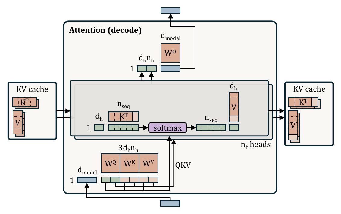
Attention during decode
These differences result in our matrices having different shapes. Where we previously had a large batch of \(b\) tokens, we now only have a single vector \((b=1)\) to multiply with our weight matrices, both for the input and output projections. Those vector-matrix multiplications are memory-bandwidth bound.
It doesn’t get better for the attention heads. Per head, the \(Q\) vector is multiplied with the \(K\) matrix and after applying the softmax operation, the resulting vector is again multiplied with the \(V\) matrix. All matrix-vector operations. Note that the parts of the \(K\) and \(V\) matrices that correspond to the past tokens (i.e. prompt tokens and tokens generated in earlier decode steps) are loaded from the KV cache.
The \(K\) and \(V\) matrices are then updated with the entry of the currently processed token. This means that the \(K\) and \(V\) matrices in the KV cache grow linearly with the number of context tokens, which means that the decode step becomes slower for every new token that is added to the sequence.
A solo session will typically leave a GPU severely underutilized because both FFN and attention are memory-bandwidth-bound during decode. As we saw for the FFN, we can bring those layers into a more compute-bound regime by batching multiple users. Can we do the same for the attention mechanism?
The Attention Mechanism: Multi-user Decode
When decoding for multiple users, the attention mechanism receives multiple input tokens. This may appear similar to prefill, but there is an important difference: during decode, the \(b\) input tokens belong to \(b\) different sequences, whereas during prefill, the input tokens belong to the same sequence. Tokens from different users do not interact with each other. Instead, each token gets information from the past tokens in its own sequence, whose keys and values are stored in that user’s KV cache. The core attention head computations therefore remain separate for each user and they remain memory-bandwidth-bound matrix-vector operations.
However, there is some benefit to batching: the input projections, involving weight matrices \(W^{Q}\), \(W^{K}\), and \(W^{V}\) as well as the output projection, involving \(W^{O}\), can be expressed as matrix-matrix multiplications by stacking the input tokens from the different users.
As a result, batched decoding improves performance through weight reuse, but attention will always be bottlenecked by the memory bandwidth required to read the KV cache. Especially so for long contexts.
Batching: Decode in company
The above is why inference servers rarely decode for a single user. They instead run batched decoding, generating one new token for each of \(b\) parallel sequences, all in the same compute step. Only one thing changes, the dimension of the input is not a vector with \(d_{model}\) elements but a genuine \(b\times d_{model}\) dimensional matrix. With this small change, the \(Q,K,V\) operations are honest matrix-matrix multiplications again. We still need to read the same info from memory, but we reuse it in \(b\) computations — the same reason that kept FFN and prefill in compute-bound territory. Similarly, the attention computations for the \(b\) sequences can be executed together.
There is a difference though. You don’t want other people to influence your results and vice-versa, so users all come with their own private part of the KV cache. The model therefore still has to read the cached keys and values for all active sequences. As a result, batched decoding improves parallelism and weight reuse, but attention can still remain limited by the memory bandwidth required to read the KV cache, especially for long contexts. In such situations, memory-bandwidth continues to be the bottleneck.
| Situation | Value of \(b\) or \(\ell\) | Typical attention regime |
|---|---|---|
| Prefill for long prompt | \(\ell\gg1\) | compute-bound |
| Prefill for multiple prompts | \(\ell\gg1\) | compute-bound |
| Single-user decoding | \(b=1\) | memory-bandwidth-bound |
| Batched decoding, short contexts | \(b\gg1\) | compute-bound |
| Batched decoding, long contexts | \(b\gg1\) | memory-bandwidth-bound |
Putting it all together:
the core trade-off
Combine the pieces and you can predict tokens per second from just the model’s dimensions and two hardware numbers — peak compute and memory bandwidth. What falls out is a trade-off: batch more requests for throughput, or keep each reply snappy — one GPU can’t maximise both.
Putting everything together, we can predict the performance of an LLM inference engine, expressed as the number of generated tokens per second, by decomposing the workload into the required matrix–matrix and matrix–vector operations. Then, plug in model dimensions and hardware specs \(C_{peak}\) and \(B_{mem}\), compute \(T_{mem}\) and \(T_{comp}\), and take the maximum of those for each operation.
For example, the table below lists the model parameters for Llama 3-8B.
| Parameter | Symbol | Llama 3-8B |
|---|---|---|
| Number of transformer layers | \(n_{layer}\) | 32 |
| Model dimension | \(d_{model}\) | 4096 |
| FFN dimension | \(d_{ff}\) | 14336 |
| Number of attention heads | \(n_{h}\) | 32 |
| Number of key-value heads | \(n_{kv}\) | 8 |
| Attention head dimension | \(d_{h}=d_{model}/n_{h}\) | 128 |
| Vocabulary size | \(V\) | 128256 |
With this info, we can estimate the runtime of each operation as a function of the context length \(\ell\) and the number of concurrent users \(b\).
This immediately shows the core trade-off between interactivity and throughput.
Throughput vs interactivity — H100 NVL, Llama 3-8B
The horizontal axis shows the interactivity, expressed as tokens per second per user. This is the performance metric perceived by an individual user, who would like to be as far to the right of the graph as possible.
The vertical axis shows the total throughput, expressed as the total number of tokens generated per second across all users. An inference provider, who typically charges per generated token, would like to operate as high as possible in the graph. The more to the left, the better the hardware is used.
The two most important variables are the average context length and the number of concurrent users. The context length is largely dictated by the intended application: a chatbot typically requires a shorter context than an agentic application that keeps track of a longer interaction history. The number of concurrent users, on the other hand, can be controlled by the inference provider.
Back to the two different regimes. For a single user, interactivity is high, but throughput is low. In this regime, the workload is severely memory-bandwidth-bound because most operations are matrix–vector operations. Remember, the model weights have to be streamed from memory to the compute units to generate only a single output token. For an inference provider, this is an inefficient operating point.
As the number of concurrent users increases, the FFN and some parts of the attention mechanism become less memory-bandwidth-bound. The model processes \(b\) new tokens at once, one per user, and the same model weights are reused across these tokens. Several operations therefore shift from matrix–vector to matrix–matrix form. As a result, throughput increases rapidly, while interactivity decreases only modestly. This is the preferred operating region for inference providers.
When the number of users keeps increasing, the cost of the KV cache becomes increasingly important. Each user request has its own KV cache, and reading the cached keys and values remains memory-bandwidth-bound. At large batch sizes and/or large context sizes, the system therefore spends an increasing fraction of time streaming KV cache data and becomes memory-bandwidth-bound again. In this region, interactivity decreases rapidly, while throughput improves only marginally. Even though the total throughput is high, the individual user experience becomes poor, making this again an undesirable operating point.
The roofline model can be a useful indicator of real inference performance. It also enables practical what-if analyses. For example, how does performance change when replacing the dense Qwen3.6-27B model with the mixture-of-experts Qwen3.6-35B-A3B model?
This is relevant for hardware owners who want to assess the feasibility of running certain models on their systems. Conversely, companies considering new hardware can use such modeling to compare different accelerator generations or vendors, such as NVIDIA and AMD. For software developers, roofline modeling helps reveal whether individual kernels approach the hardware limits or run at suboptimal speed. Finally, for chip designers and system integrators, it helps answer architectural questions, such as how changing the memory bandwidth would affect overall inference performance.
Conclusion
The plot shows that roofline modeling is a useful indicator of real inference performance. It gives insight into how a workload maps onto the underlying hardware and where it hits a bottleneck. This is especially powerful combined with real measurements. When a measurement drifts away from the estimate, that gap helps diagnose performance issues and improve the system’s latency or throughput. We’ll deep-dive into the most relevant bottlenecks for LLM inference in follow-up posts so stay tuned!
References
- Poetry Foundation (Edgar Allan Poe), “The Raven” poetryfoundation.org
- Sebastian Raschka, “How to build an LLM from scratch” sebastianraschka.com. We also highly recommend his blog magazine.sebastianraschka.com
- Meta, “Llama 3 Model Card” github.com
- Further reading: for an excellent deep-dive into these topics, “How to Scale Your Model” jax-ml.github.io


Join the conversation
We publish every aistack insight on LinkedIn — add your read, push back on the benchmarks, or follow along for the next one.
Discuss on LinkedIn